This work was done during the Quantum Open Source Foundation mentorship program, Cohort 9. I would like to express my gratitude to my mentor Danial Motlagh and to QOSF.

Introduction

Catalytic processes are the workhorses of industry – for example, the Haber–Bosch synthesis of ammonia $\text{N}_2 + 3\text{H}_2 \overset{\text{Fe}}{\longrightarrow} 2\text{NH}_3$ runs under extreme conditions and consumes roughly 1% of the world’s energy supply.

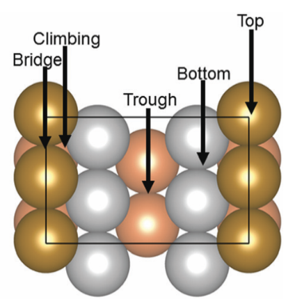
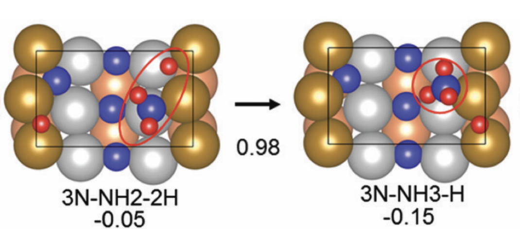
Understanding the reaction pathway with catalyst hopes to gain insights into the process, enhancing its efficiency. [1] has simulated the reaction using VASP using Fe211 as a catalyst as shown in Fig. 1. However, classical simulation methods like VASP quickly become forbiddenly expensive as the system grows, whereas quantum algorithms have long been predicted to outperform classical computers in modeling complex chemical processes. Indeed, hybrid quantum–classical approaches offer a natural way to handle the many-body quantum chemistry and the classical geometry search in tandem. By offloading the hardest electronic-structure parts to a quantum processor, we can efficiently evaluate energies for different molecular configurations, then use classical routines to adjust positions and orientations.

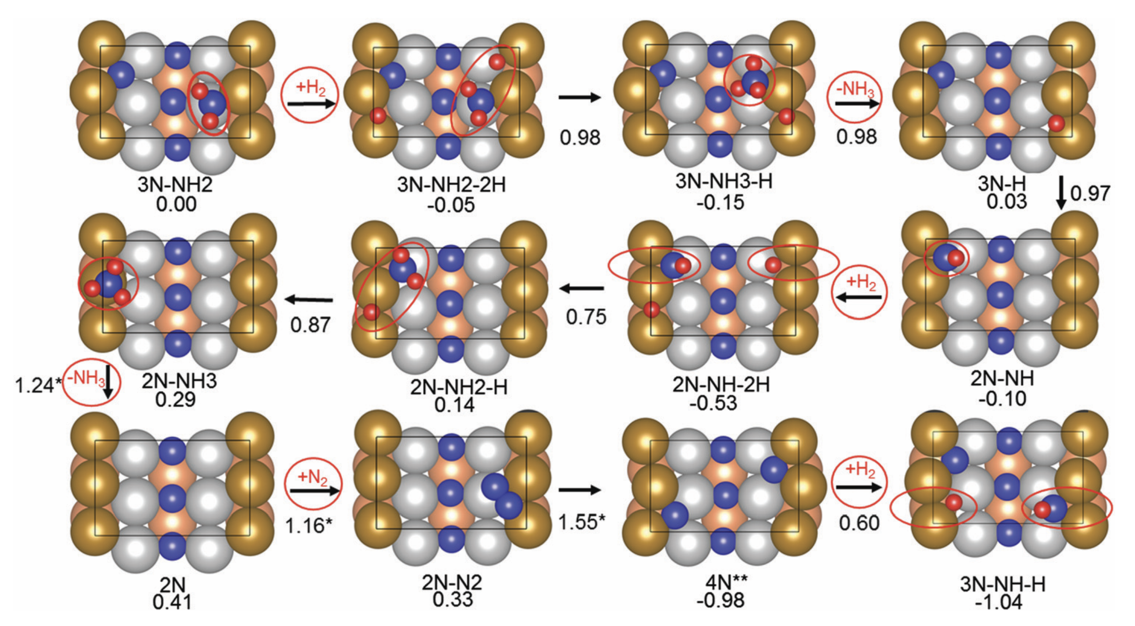
This post explores how we can use Pennylane to execute the first steps with limited computer resources. Concretely, we replicate the first three steps of [1] in Fig. 2, which are the most complex reactions in the whole pathway. It is computationally cheaper than the method used in [1].

Method

1. Varies the coordinates of the reactant: The transition in $x,y,z$ axis and rotation angle around its center.
   • We use two optimization methods: Gradient descent and Bayesian optimization (BO). The former method has good coverage in these Pennylane demoes in a 1D setup.
   • In this work, we focus on the latter in a 3D setup. For a comprehensive review of BO, we refer readers to [3].
2. Construct the Hamiltonian
3. Measure and Optimize: Measure the expectation value of the Hamiltonian using the quantum circuit and optimize the parameters using a classical optimizer to minimize this value.

Motivation

To define a 3D affine transformation for a molecule, we need to define three translation parameters $t_x, t_y, t_z$ and three rotational parameters $\theta_x,\theta_y,\theta_z$. Calculating the gradient needs $t_\bullet \pm \Delta_t$ and $\theta_\bullet \pm \Delta_\theta$. Therefore, each learning step requires $6 \times 2$ Hamiltonian, which is expensive.

Bayes Optimization (BO)

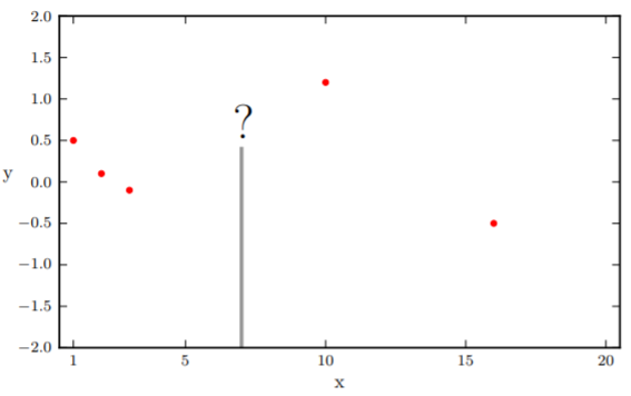
BO, being a gradient-less method, does not have these requirements. Here is how it works. After the initial samplings $\pmb{X}=x_1, x_2, ... , x_n$ , Gaussian processing (GP) assume that

$\pmb{X} \sim \mathscr{N}\begin{bmatrix}\begin{pmatrix} \mu_1 \\ \vdots \\ \mu_n\end{pmatrix},\begin{pmatrix}1 & K_{12} & \cdots & K_{1n}\\ K_{21} & \vdots & \ddots & \vdots \\ K_{n1} & K_{n2} & \cdots & K_{nn} \end{pmatrix} \end{bmatrix}$

and fixes a regression curve through these data points. Only the observed data points have absolute certainty (variance = 0). For an unknown point $x'$, GP returns a prediction from the distribution of $\mathscr{N}(\mu,\Sigma\lvert\pmb{X})$.

A beautiful property of Gaussian is that when conditioning the Gaussian on a set of variables, the result is also a Gaussian $\mathscr{N}(\mu',\Sigma')$. In Fig.2, the prediction value of the unknown point is $\mu'$, whereas the confidence interval is $\Sigma'$.

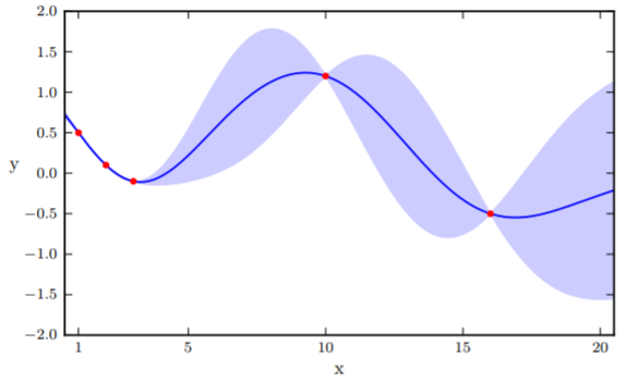
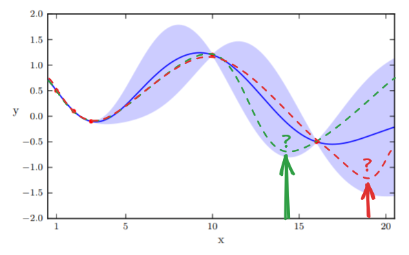
Here, we face a dilemma. In $\pmb{X}$ there is a point with the smallest value $x_{min}$. Therefore, the next minima should be somewhere close to it. However, it is also possible that points in the wide confidence interval have smaller values than the current minima. To quantify this trade-off, we define an acquisition function $\alpha$ to obtain new positions to sample. There are several approaches to define $\alpha$, we are using the Expected Improvement (EI) approach here.

EI works by generating random functions that lie inside the confident intervals, as demonstrated in Figure 3. The intuition is a larger confidence interval would have more diverse sampling functions. Afterward, we sample the point at the extrema and update the prior. The process continues for a predefined number of steps.

Simplification

To facilitate the calculation with our limited computing resources we made the following simplification

1. Calculating the Hamiltonian with $\text{STO-3G}$, a minimal orbital basis.
2. Simplyfing the catalyst substrate.

Visualization

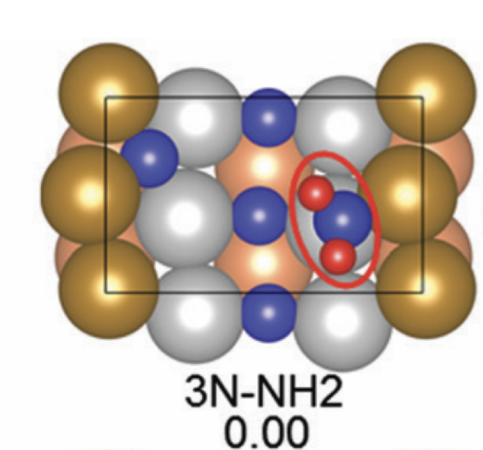
We will replicate the first three steps of Figure 2, whose Hamiltonians are the most complex in the whole pathway.

In the below visualization, we color-coded the atoms as $\text{Fe}$ $\text{N}$ , and $\text{H}$ . Please open the GIFs/videos in a new tab for a full-resolution version.

Step 1

We fix the coordinates of the catalyst substrate and use the gradient descent method to optimize the coordinates of the reactants. The result is as follows.

Even with the same learning rate, the speed of the reactants slows down greatly compared to the beginning. Therefore, we conclude that in this step, the learning converged.

Step 2

In this step, we add $H_2$ as a reactant. To minimize the time to build the Hamiltonian, we fix the coordinates of all the reactants of the previous step. Since gradient descent works before, let’s apply the same method.

Note the moving speed of the reactants is much slower than the previous step. Therefore, it is clear that we are stuck at a local minimum, and gradient descent would have a hard time escaping it without modeling the endothermicity of this reaction ($$0.98$$ below the arrow). Let us try with BO to see if it can overcome this minima. Due to the nature of the acquisition function, the plot of the ground state energy does not decrease nicely as seen in the gradient descent. Most of the $$\text{H}$$ atoms went too far away from the catalyst substrate, due to our initial setup of the search margin, which is $$1 nm$$ bigger than the catalyst substrate. Here we filter only what went inside the substrate.

We conclude that the search boundary condition is of utmost importance. Accordingly, we modify the search space as below.

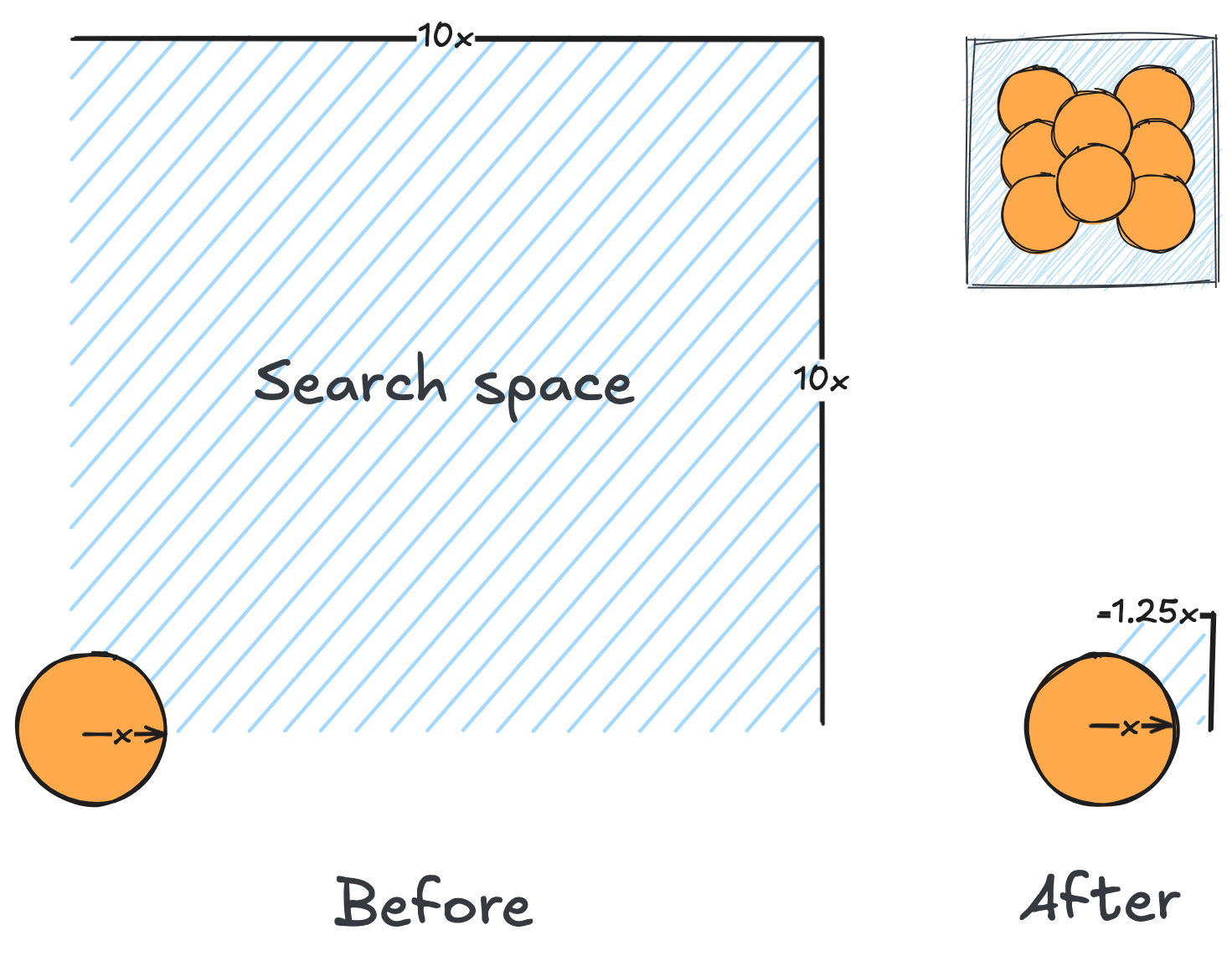
Here is the optimization after setting the search boundary. We made these demonstration videos instead of GIFs so that readers can control the frame shown.

$\text{NH}_3$ molecule is produced in a total of 6 trials (namely 12th, 13th, 25th, 26th, 27th, and 28th), which coincidentally matches the efficiency of the Harber-Bosch process of about 20%¹. It also offers an explanation for that number, which is the coordinates that create $\text{NH}_3$ have higher ground state energy than the other configurations where $\text{H}$ atoms float away. Note that there are times that the BO chooses to sample two very close points consecutively (12th and 13th frame for example), it is because of the exploitation and exploration trade-of that we mentioned earlier

Conclusion

This blog post provides an alternate method to optimize the geometry of the Haber-Bosch process. Due to the lack of computational resources we have to reduce the catalyst platform, number of active orbitals, and electrons. These parameters are visible in chem_config.yaml. Even with a simple orbital basis and reduced numbers of active electrons and orbitals, the experiments still take up a lot of time.

• Gradient descent: 32 CPU, 256 GB RAM, 50h runtime
• BO: 8 CPU, 64 GB RAM, 60h runtime

The parameters of free electrons and free orbitals are crucial parameters to make this project possible as a full configuration interaction can take up to TBs of RAM to calculate. That being said, our current simple setup can replicate the location where $\text{NH}_3$ is produced on the catalyst surface.

Comments? Questions? Please let us know at Issues page

References

[1] Reaction mechanism and kinetics for ammonia synthesis on the Fe(211) reconstructed surface. Jon Fuller, Alessandro Fortunelli, William A. Goddard III, and Qi An. Physical Chemistry Chemical Physics Issue 21, 2019

[2] Reiher Markus, Nathan Wiebe, Krysta M. Svore, Dave Wecker and Matthias Troyer. Elucidating reaction mechanisms on quantum computers. Proceedings of the National Academy of Sciences 2017

[3] Kevin Patrick Murphy. Machine Learning: a Probabilistic Perspective. MIT Press, 2012

Footnotes

1. https://en.wikipedia.org/wiki/Haber_process#Ammonia_production ↩